Chris IJ Hwang
I am a Quantitative Analyst/Developer and Data Scientist with backgroud of Finance, Education, and IT industry. This site contains some exercises, projects, and studies that I have worked on. If you have any questions, feel free to contact me at ih138 at columbia dot edu.
Contents
Smart Beta Strategy
There are many different factors and smart beta strategies. In this report, I want to focus on how utilize the different portfolio construction.
Previously, I have used data and platform from quantopian.com. This time, I have constructed my platform on Amazon Web Services(AWS) using Linux server along with MySQL database.
import pandas as pd
import numpy as np
import seaborn as sns
import matplotlib.pyplot as plt
%matplotlib inline
from ch_api import ch_optimize, util, ch_portfolio

import importlib
USE_DB = True  # It DB connection is limited, let's use pickle files inluced in the repo not connecting DB
ID = ''
PW = ''
import yaml
from sqlalchemy import create_engine


engine = create_engine('mysql+pymysql://%s:%s@localhost/securities_master' %
                       (ID, PW),
                       echo=False)
Data
Universe of SP 500
Daily price data of SP 500 are collected from yahoo finance.
Factors
I used factors from the Fama_Frent 5 factor models and Momentum from the data library in the site (http://mba.tuck.dartmouth.edu/pages/faculty/ken.french/data_library.html)
See this (http://mba.tuck.dartmouth.edu/pages/faculty/ken.french/Data_Library/f-f_5_factors_2x3.html) for 5 factor model and here (http://mba.tuck.dartmouth.edu/pages/faculty/ken.french/Data_Library/det_mom_factor.html) for momentum factor defiine.
if USE_DB:
    factors_ts = pd.read_sql("select * from symbol where instrument='factor' and ticker<>'RF'", engine)
    # factors data are available in the pickle file: %root%/input/factors.pkl
    #factors_ts.to_pickle("../data/factors.pkl")
else:
    factors_ts = pd.read_pickle('../data/factors.pkl')

tis = list(factors_ts['ticker'].values)
# Factors
tis
['Mkt-RF', 'SMB', 'HML', 'RMW', 'CMA', 'MOM']
Platform
Python 3.7 and CVXPY are the key components. Please refer to the file %project_root%/python_environment.txt

Beta, Loading, and Covariance
For this project, I used 250-day lookback period for rolling daily loading value of Beta, factor loadings, and covarianace/correlation computation.
See
%project_root%/clients/market_beta.py
%project_root%/clients/factor_loading.py
Factors Performance & Correlation
start_date = '2012-01-02'
end_date = '2018-08-24'

if USE_DB:
    stm = "select * from daily_price where ticker in %s and instrument_type='factor'" % str(tuple(tis))
    factors_ts = pd.read_sql(stm, engine)

    factors_ts = factors_ts[['price_date', 'ticker', 'adj_close_price']]
    idx = (factors_ts['price_date']>=start_date) & (factors_ts['price_date']<=end_date)

    df_sliced = factors_ts[idx].copy()
    df_sliced.set_index(['price_date', 'ticker'],inplace=True)
    factors_unstacked = df_sliced.unstack(level=-1)
    factors_unstacked_aligned = factors_unstacked.dropna()
    #factors_unstacked_aligned.to_pickle("../data/factors_return.py")
else:
    factors_unstacked_aligned = pd.read_pickle("../data/factors_return.py")
factors_unstacked_aligned.head()
| adj_close_price | ||||||
|---|---|---|---|---|---|---|
| ticker | CMA | HML | MOM | Mkt-RF | RMW | SMB |
| price_date | ||||||
| 2012-01-03 | -0.0021 | 0.0087 | -0.0261 | 0.0150 | -0.0067 | -0.0010 |
| 2012-01-04 | -0.0005 | 0.0009 | 0.0012 | 0.0000 | 0.0026 | -0.0063 |
| 2012-01-05 | 0.0008 | 0.0014 | -0.0058 | 0.0039 | -0.0038 | 0.0020 |
| 2012-01-06 | -0.0004 | -0.0026 | -0.0006 | -0.0019 | -0.0004 | -0.0004 |
| 2012-01-09 | 0.0025 | -0.0005 | -0.0034 | 0.0028 | -0.0021 | 0.0027 |
factors_unstacked_aligned = factors_unstacked_aligned['adj_close_price'].copy()
factors_unstacked_aligned_cum = np.cumprod(factors_unstacked_aligned + 1.0) - 1.0
factors_unstacked_aligned_cum.to_csv("../output/factors_cum_returns.csv")

sns.heatmap(factors_unstacked_aligned.corr(), annot=True)
<matplotlib.axes._subplots.AxesSubplot at 0x7f8f87d68f60>
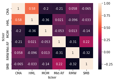
Overview Scenario
Value and Momentum is known as historically negative correlation. The target horizon for this analysis if from 2017/1/4 ~ 2017/12/30. During this period, Value factor was in downturn and Momentum factor return is going up while it was opposite during year 2016.
First, I will construct 4 different portfolio for different goals but using same stocks with different weights scheme.
There are four different portfolio constructed.
- portfolio 1. Value long-only portfolio
- portfolio 2. Value + Momentum long-onluy portfolio
- portfolio 3. Equal weight long-only portfolio
- portfolio 4. Min Variance long-only portfolio
Since we already know that during 2017, value return was negative while momemtum and market were positive. The portfolio 1 is expected to be negative, but we will see how much the portfolio 2 which is combined with momentum will be helpful. All portfolio will be rebalanced daily.
Base Portfoliio
The first baseline portfolio is equal weight portfolio with stocks randomly selected from each sector.
Its asset level information is below:
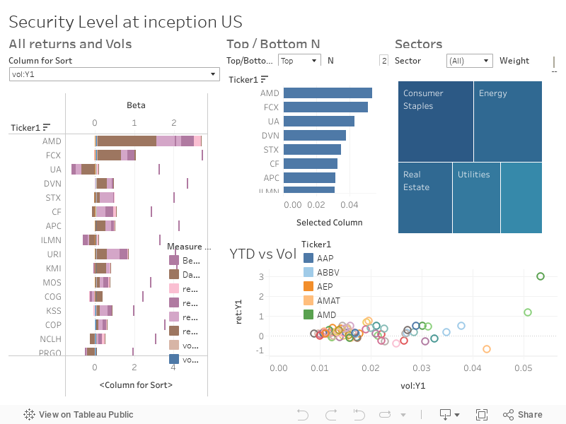
Portfolios
- Equal Weight (ew_pf_all)
- Mean Variance (MV)
- Value (Value)
- Value + Momentum (Value_Mom)
1. Baseline portfolio: Equal Weight Portfolio
ew_portfolio_ts = pd.read_pickle('../output/ts_base_portfolio.pkl')
ew_portfolio_ts.rename(columns={'metric_date': 'date'}, inplace=True)
ew_portfolio_ts.set_index(['date', 'ticker'], inplace=True)
ew_portfolio_ts.head()
| CMA | HML | MOM | Mkt-RF | RMW | SMB | beta | daily_return | inception_date | name | pf_name | price | sector | weight | ||
|---|---|---|---|---|---|---|---|---|---|---|---|---|---|---|---|
| date | ticker | ||||||||||||||
| 2017-01-04 | UA | -1.3362 | 0.3133 | -0.9523 | 0.8744 | -0.3100 | 0.2990 | 1.6032 | 0.0314 | 2017-01-04 | Under Armour Class C | ew_pf_all | 26.5700 | Consumer Discretionary | 0.0141 |
| AAP | 0.4638 | -0.0423 | 0.3011 | 1.1246 | 0.5644 | 0.2373 | 0.9311 | 0.0082 | 2017-01-04 | Advance Auto Parts | ew_pf_all | 171.4716 | Consumer Discretionary | 0.0141 | |
| KSS | 0.7001 | 0.3590 | -0.0257 | 0.8332 | 0.9086 | 1.2936 | 0.9613 | 0.0422 | 2017-01-04 | Kohl's Corp. | ew_pf_all | 47.7039 | Consumer Discretionary | 0.0141 | |
| LEN | -0.4864 | 0.2597 | -0.1227 | 1.1653 | 0.7193 | 0.3950 | 1.2897 | 0.0247 | 2017-01-04 | Lennar Corp. | ew_pf_all | 43.0236 | Consumer Discretionary | 0.0141 | |
| DHI | -0.6686 | 0.2399 | 0.1262 | 1.4062 | 0.4596 | 0.3211 | 1.4566 | 0.0243 | 2017-01-04 | D. R. Horton | ew_pf_all | 27.6662 | Consumer Discretionary | 0.0141 |
ew_portfolio_ts.tail()
| CMA | HML | MOM | Mkt-RF | RMW | SMB | beta | daily_return | inception_date | name | pf_name | price | sector | weight | ||
|---|---|---|---|---|---|---|---|---|---|---|---|---|---|---|---|
| date | ticker | ||||||||||||||
| 2017-12-29 | SO | 0.1923 | -0.2192 | 0.0853 | 0.1449 | 0.1820 | -0.4436 | -0.0128 | -0.0039 | NaN | Southern Co. | ew_pf_all | 46.2199 | Utilities | 0.0141 |
| FE | 0.5098 | -0.3313 | -0.0613 | 0.3937 | 0.1132 | -0.6176 | 0.0896 | 0.0056 | NaN | FirstEnergy Corp | ew_pf_all | 29.6545 | Utilities | 0.0141 | |
| LNT | 0.1568 | -0.2446 | -0.0118 | 0.3417 | 0.3191 | -0.3614 | 0.1800 | -0.0012 | NaN | Alliant Energy Corp | ew_pf_all | 41.5924 | Utilities | 0.0141 | |
| NI | 0.3920 | -0.3680 | 0.0091 | 0.5732 | 0.3117 | -0.5431 | 0.3441 | 0.0043 | NaN | NiSource Inc. | ew_pf_all | 25.0607 | Utilities | 0.0141 | |
| DUK | 0.0537 | -0.0941 | -0.0310 | 0.2038 | 0.2062 | -0.4132 | 0.0302 | 0.0014 | NaN | Duke Energy | ew_pf_all | 81.2140 | Utilities | 0.0141 |
portfolio returns
# portfolio returns
port_ret = ew_portfolio_ts.groupby(level=0).apply(lambda x: (x['weight']*x['daily_return']).sum())
port_ret_df = pd.DataFrame(port_ret)
port_ret_df.columns = ['EW']
port_ret_df.head()
| EW | |
|---|---|
| date | |
| 2017-01-04 | 0.011033 |
| 2017-01-05 | -0.001981 |
| 2017-01-06 | 0.000398 |
| 2017-01-09 | -0.007755 |
| 2017-01-10 | 0.001308 |
portfolio exposures
ew_portfolio_ts_reset = ew_portfolio_ts.reset_index()

exposure_ts_df = ew_portfolio_ts_reset.groupby('date').apply(lambda x: ch_portfolio.computing_exposures(x))
exposure_ts_df.head()
| sector | Consumer Discretionary | Consumer Staples | Energy | Financials | Health Care | Industrials | Information Technology | Materials | Real Estate | Telecommunication Services | Utilities | date | portfolio_name | CMA | HML | MOM | Mkt-RF | RMW | SMB | |
|---|---|---|---|---|---|---|---|---|---|---|---|---|---|---|---|---|---|---|---|---|
| date | ||||||||||||||||||||
| 2017-01-04 | 0 | 0.0846 | 0.141 | 0.1269 | 0.0705 | 0.0705 | 0.0705 | 0.0846 | 0.0987 | 0.1269 | 0.0141 | 0.1128 | 2017-01-04 | ew_pf_all | 0.485095 | -0.142093 | -0.173468 | 1.038622 | 0.185378 | -0.061437 |
| 2017-01-05 | 0 | 0.0846 | 0.141 | 0.1269 | 0.0705 | 0.0705 | 0.0705 | 0.0846 | 0.0987 | 0.1269 | 0.0141 | 0.1128 | 2017-01-05 | ew_pf_all | 0.480883 | -0.137318 | -0.171566 | 1.037753 | 0.187069 | -0.057236 |
| 2017-01-06 | 0 | 0.0846 | 0.141 | 0.1269 | 0.0705 | 0.0705 | 0.0705 | 0.0846 | 0.0987 | 0.1269 | 0.0141 | 0.1128 | 2017-01-06 | ew_pf_all | 0.486516 | -0.135081 | -0.167447 | 1.040831 | 0.194314 | -0.056110 |
| 2017-01-09 | 0 | 0.0846 | 0.141 | 0.1269 | 0.0705 | 0.0705 | 0.0705 | 0.0846 | 0.0987 | 0.1269 | 0.0141 | 0.1128 | 2017-01-09 | ew_pf_all | 0.490078 | -0.133538 | -0.162041 | 1.045910 | 0.190487 | -0.055758 |
| 2017-01-10 | 0 | 0.0846 | 0.141 | 0.1269 | 0.0705 | 0.0705 | 0.0705 | 0.0846 | 0.0987 | 0.1269 | 0.0141 | 0.1128 | 2017-01-10 | ew_pf_all | 0.486553 | -0.131016 | -0.158807 | 1.047882 | 0.190611 | -0.050869 |
2. other three portfolios
- MinVariance : %project_root%/cfg/mv.py
- Value tilt: %project_root%/cfg/value.py
- Value + Momentum tilt: %project_root%/cfg/value_mom_mix.py
importlib.reload(ch_optimize)
<module 'ch_api.ch_optimize' from '/home/ec2-user/work/QuantResearch/ch_api/ch_optimize.py'>
# optimize each portfolio with daily rebalancing
# 1. portfolio return df : port_ret_df
# 2. portfolio exposure df: exposure_ts_df
from cfg import mv, value, value_mom_mix
lst_portfolio = [mv, value, value_mom_mix]
for pf in lst_portfolio:
    # 1. optimize ts data
    opt = ch_optimize.Optimizer().createOptimizer(pf,
                                optimizer_type='MV', engine=engine,
            lst_factor=[ u'CMA', u'HML', u'MOM', 'RMW',u'SMB',])
    optimized_df = opt.run_optimize(ew_portfolio_ts)
    optimized_df = optimized_df.rename(columns={
        'weight': 'old_weight',
        'optimized_weight': 'weight'})
    optimized_df['pf_name'] = pf.pf_name

    # 2. shift optimized_weight
    opt_weights_sr = optimized_df.unstack()['weight'].shift().stack()
    opt_weights_df = pd.DataFrame(opt_weights_sr)
    opt_weights_df.columns = ['optimized_weight_shift']
    final_portfolio = optimized_df.merge(opt_weights_df,
                                           left_index=True,
                                           right_index=True,
                                           how='left')
    # 3. performance computation
    final_portfolio_perf = final_portfolio.groupby(level=0).apply(
        lambda x: (x['daily_return'] * x['optimized_weight_shift']).sum())
    final_portfolio_perf_df = pd.DataFrame(final_portfolio_perf)
    final_portfolio_perf_df.columns = [pf.pf_name]
    port_ret_df= pd.concat([port_ret_df, final_portfolio_perf_df], axis=1)
    # 4. Exposure computation
    final_portfolio_exp_ready = final_portfolio.rename(columns={'weight': 'optimized_weight',
                                                      'optimized_weight_shift': 'weight'})

    final_portfolio_exp_ready_reset = final_portfolio_exp_ready.reset_index()
    exposure_ts_tmp_df = final_portfolio_exp_ready_reset.groupby('date').apply(
                 lambda x: ch_portfolio.computing_exposures(x))


    exposure_ts_df = pd.concat([exposure_ts_df, exposure_ts_tmp_df])
exposure_ts_df['portfolio_name'].unique()
array(['ew_pf_all', 'MV', 'Value', 'Value_Mom'], dtype=object)
exposure_ts_df.to_csv('../output/exposure_ts_df_total.csv')
port_ret_df.head()
| EW | MV | Value | Value_Mom | |
|---|---|---|---|---|
| date | ||||
| 2017-01-04 | 0.011033 | 0.000000 | 0.000000 | 0.000000 |
| 2017-01-05 | -0.001981 | -0.001029 | -0.008573 | -0.005672 |
| 2017-01-06 | 0.000398 | -0.000776 | 0.006222 | 0.004171 |
| 2017-01-09 | -0.007755 | -0.007129 | -0.008989 | -0.006686 |
| 2017-01-10 | 0.001308 | 0.005204 | 0.009201 | 0.012008 |
vol_df = pd.DataFrame(port_ret_df.std() * np.sqrt(250))
vol_df.columns = ['Vol']
vol_df
| Vol | |
|---|---|
| EW | 0.072797 |
| MV | 0.075962 |
| Value | 0.160162 |
| Value_Mom | 0.104974 |
final_return_df = pd.DataFrame(port_cum_ret_df.iloc[-1])
final_return_df.columns = ['Return']
final_return_df
| Return | |
|---|---|
| EW | 0.176100 |
| MV | 0.175094 |
| Value | -0.035823 |
| Value_Mom | 0.108284 |
summary_df = pd.concat([final_return_df, vol_df], axis=1)
summary_df
| Return | Vol | |
|---|---|---|
| EW | 0.176100 | 0.072797 |
| MV | 0.175094 | 0.075962 |
| Value | -0.035823 | 0.160162 |
| Value_Mom | 0.108284 | 0.104974 |
summary_df['Risk Adj Ret'] = summary_df['Return']/summary_df['Vol']
summary_df
| Return | Vol | Risk Adj Ret | |
|---|---|---|---|
| EW | 0.176100 | 0.072797 | 2.419046 |
| MV | 0.175094 | 0.075962 | 2.305025 |
| Value | -0.035823 | 0.160162 | -0.223667 |
| Value_Mom | 0.108284 | 0.104974 | 1.031536 |
port_cum_ret_df = np.cumprod(port_ret_df + 1.0) - 1.0
port_cum_ret_df.to_csv('../output/port_cum_ret_df_total.csv')
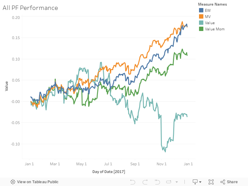
Portfolio Returns
Portfolio Factor Sensitity

Portfolio Sector Exposures

Summary
As expected, value portfolio was the worst performer. Value_Mom portfolio has boosted much better while both equal weighted and Min variance portfolio had good risk adjusted returns. In case of MV portfolio, its exposure to all factors except Market-Riskfree are mostly between -0.1 ~ 0.15.
For the further analysis, it should be done using stock selection methods for each portfolio especially Value-Momentum portfolio with different mix and integration methods.
References
Israel, Ronen and Jiang, Sarah and Ross, Adrienne, Craftsmanship Alpha: An Application to Style Investing (September 8, 2017). Available at SSRN: https://ssrn.com/abstract=3034472 or http://dx.doi.org/10.2139/ssrn.3034472
Fama, Eugene F. and French, Kenneth R., A Five-Factor Asset Pricing Model (September 2014). Fama-Miller Working Paper. Available at SSRN: https://ssrn.com/abstract=2287202 or http://dx.doi.org/10.2139/ssrn.2287202
Equity factor-based investing: A practitioner’s guide. https://www.vanguardinvestments.com.au/adviser/adv/articles/insights/research-commentary/portfolio-construction/factor-based-investing.jsp##whats-worked